Predictive maintenance is revolutionizing industrial operations by enabling companies to anticipate equipment failures before they happen. By leveraging machine learning techniques, businesses can significantly reduce downtime and maintenance costs, ensuring smoother and more efficient operations. One such technique is the Isolation Forest algorithm, which excels in identifying anomalies within datasets.

In the first part of our Anomaly Detection 101 series, we learned the fundamentals of Anomaly Detection and saw how spectral clustering can be used for credit card fraud detection. This method helps in identifying fraudulent transactions by grouping similar data points and detecting outliers. Building on that foundation, we now turn our attention to predictive maintenance. In this tutorial, you will learn how to implement a predictive maintenance system using the Isolation Forest algorithm — a well-known algorithm for anomaly detection.

This lesson is the 2nd of a 4-part series on Anomaly Detection:

Credit Card Fraud Detection Using Spectral Clustering
Predictive Maintenance Using Isolation Forest (this tutorial)
Building Network Intrusion Detection System with Variational Autoencoders
Outlier Detection Using the Grubbs Test

To learn how to use Isolation Forest for predictive maintenance of machines, just keep reading.

What Is Predictive Maintenance? And Why Anomaly Detection?

Imagine you have a car, and instead of waiting for it to break down or following a strict maintenance schedule, you use sensors to monitor the engine’s performance, oil levels, and tire pressure. These sensors continuously send data to a system that analyzes the information and predicts when a part might fail. This way, you can address potential issues before they become serious problems. This is exactly what predictive maintenance is.

Predictive Maintenance

Predictive maintenance is a proactive approach to maintaining equipment and machinery by predicting when failures might occur. This method leverages data from various sensors and advanced analytics to monitor the condition of equipment in real-time.

The importance of predictive maintenance (Figure 1) cannot be overstated. It helps companies avoid unexpected equipment failures, which can lead to costly downtime and repairs. For example, in a manufacturing plant, a sudden machine breakdown can halt production, leading to significant financial losses.

**Figure 1:** Importance of predictive maintenance (source: Keepler).

By using predictive maintenance, companies can schedule repairs during planned downtime, ensuring that production continues smoothly. Additionally, this approach extends the lifespan of equipment by addressing issues early, reducing the need for frequent replacements.

Predictive Maintenance as Anomaly Detection

Predictive maintenance can be effectively posed as an anomaly detection problem (Figure 2). Anomalies are deviations from the normal behavior of a system, and in the context of predictive maintenance, they indicate potential failures or issues.

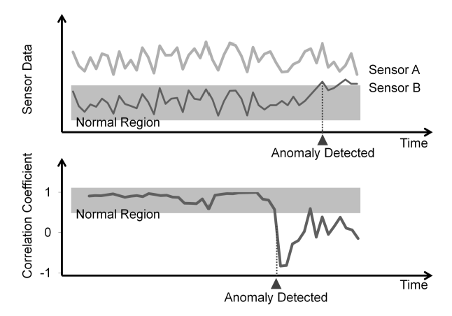
For instance, if a machine usually operates within a certain temperature range, a sudden spike in temperature could be an anomaly, signaling a problem. By continuously monitoring data from sensors, machine learning algorithms can learn the normal operating patterns of equipment and detect anomalies that may indicate impending failures.

The Isolation Forest Algorithm

Various techniques can be employed to solve predictive maintenance using anomaly detection. One common method is the Isolation Forest algorithm, which is particularly effective in identifying anomalies in large datasets.

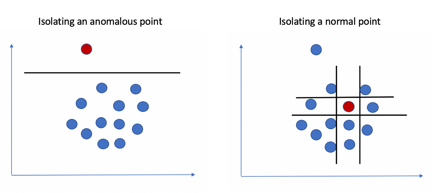
Isolation Forest is a class of Ensemble methods that combine multiple algorithms to improve the accuracy and robustness of anomaly detection. For example, in layperson terms, Isolation Forest isolates anomalies by randomly selecting a feature and splitting the data (Figure 3). Because of this, anomalies are isolated quickly because they are rare and different.

**Figure 3:** Isolation Forest isolates anomalies by randomly selecting a feature and splitting the data (source: Data Science Demystified).

In an industrial setting, if a factory uses vibration sensors to monitor machinery, the Isolation Forest algorithm can detect unusual vibration patterns that may indicate a misalignment or wear and tear.

Let’s understand the Isolation Forest algorithm in detail.

Isolation Trees

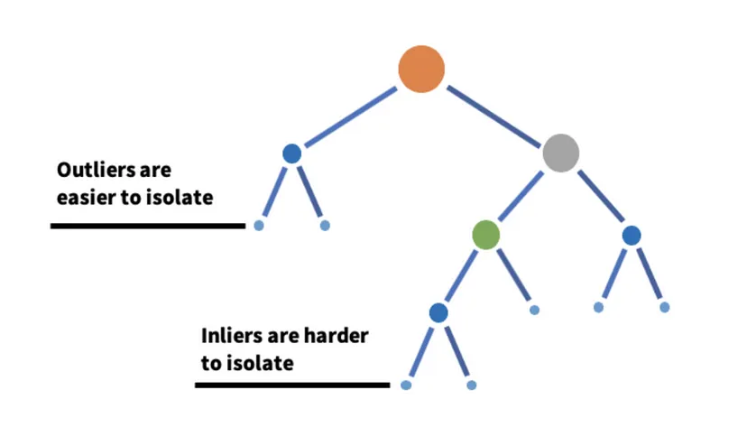
The core of the Isolation Forest algorithm is the Isolation Tree (iTree), a binary tree structure. Each tree is built by recursively partitioning the data (Figure 4). At each node, a feature is randomly selected, and a random split value is chosen between the minimum and maximum values of that feature.

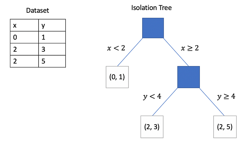
**Figure 4:** Isolation Tree is a binary tree structure built by recursively partitioning the data (source: Data Science Demystified).

Data points having feature values less than or equal to the split value go into the left subtree, while others go to the right subtree.

This process continues until each data point is isolated in its own leaf node or a predefined tree height is reached. Anomalies, being few and different, tend to be isolated quickly, resulting in shorter paths in the tree.

Anomaly Score

The anomaly score for a data point is determined by the average path length required to isolate it across all trees in the forest. The shorter the average path length, the more likely the point is an anomaly (Figure 5).

**Figure 5:** The shorter the average path length, the more likely the point is an anomaly (source: Medium).

Mathematically, the anomaly score $s(x, n)$ for a point $x$ in a dataset of size $n$ is given by:

$s(x, n) = 2^{-\frac{E(h(x))}{c(n)}}$

where $E(h(x))$ is the average path length of data point $x$ (across a set of iTrees) and $c(n)$ is the average path length of unsuccessful searches in a Binary Search Tree, approximated as:

$c(n) = 2H(n-1) - \displaystyle\frac{2(n-1)}{n}$

with $H(i)$ being the harmonic number.

Building the Forest

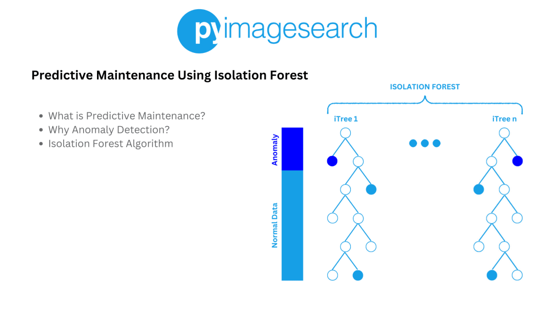
Multiple Isolation Trees are constructed to form an Isolation Forest (Figure 6). Each tree is built using a random subset of the data, enhancing the robustness of the anomaly detection process.

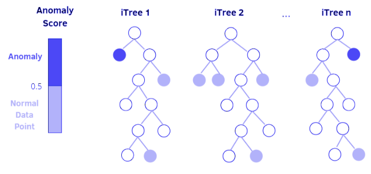
**Figure 6:** An Isolation Forest is a collection of multiple iTrees built using random subsets of data (source: Medium).

The final anomaly score for a data point is the average of its scores across all trees. Points with scores close to 1 are considered anomalies, while those with scores much lower are considered normal.

Implementing Predictive Maintenance Using Isolation Forest

In this section, we will see how we can use Isolation Forest for predictive maintenance (i.e., detection of potential failures or issues).

We will start by setting up libraries and data preparation.

Setup and Data Preparation

For this purpose, we will use the Pump Sensor Dataset, which contains readings of 52 sensors that capture various parameters (e.g., temperature, pressure, vibration, etc.) for a water pump operational in a small town. There are over 220K readings, each captured at a minute interval. Out of these 220K readings, only 7 data points have machine status as “BROKEN”, while around 14K readings have machine status as “RECOVERING”. For the remaining majority of readings, the machine status is “NORMAL”.

The goal of this mini project is to successfully predict the “RECOVERING” and “BROKEN” (considered as anomalies) status of the water pump using Isolation Forest.

To download our dataset and set up our environment, we will install the following packages.

kaggle: command line API for downloading the datasets from Kaggle
pandas: to load our dataset files
matplotlib: to plot and visualize the dataset and anomalies
scikit-learn: for computing precision and recall of the system
numpy: for numerical computation.

$ pip install kaggle pandas matplotlib scikit-learn numpy
$ kaggle datasets download -d nphantawee/pump-sensor-data
$ unzip /content/pump-sensor-data.zip -d /content/

After downloading the dataset, we will now load our pump sensor dataset, preprocess various features, and then visualize them via Matplotlib plots.

import pandas as pd
import matplotlib.pyplot as plt

data = pd.read_csv("/content/sensor.csv", header='infer')

data = data.drop(["timestamp", "Unnamed: 0"], axis=1)
type_dict = {'NORMAL': 0, 'RECOVERING': 1, 'BROKEN': 1}
data["machine_status"] = data["machine_status"].apply(lambda x: type_dict[x])

data = data.fillna(0)
print(data.head())
print(data["machine_status"].value_counts())

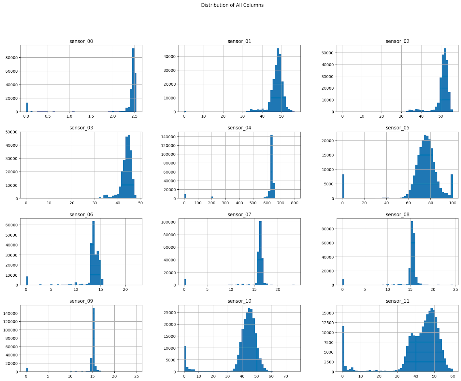
# Plotting the distribution of all columns
data.iloc[:, :12].hist(bins=50, figsize=(20, 15))
plt.suptitle('Distribution of All Columns')
plt.show()

We start by importing the necessary libraries, pandas and matplotlib.pyplot (Lines 1 and 2). We then read a CSV file named "sensor.csv" into a DataFrame called data (Line 4). Next, we drop the "timestamp" and "Unnamed: 0" columns from the DataFrame (Line 6). We create a dictionary type_dict to map the machine status values to numerical values and apply this mapping to the "machine_status" column (Lines 7 and 8). Missing values in the DataFrame are filled with zeros (Line 10), and we print the first few rows of the DataFrame and the value counts of the "machine_status" column (Lines 11 and 12).

Finally, we plot the distribution of the first 12 columns in the DataFrame using histograms (Lines 15-17). The histograms are displayed in a grid with 50 bins each, and the overall plot is given the title 'Distribution of All Columns'. This helps us visualize the data distribution across different columns.

Figure 7 shows the distribution of various sensor readings in the dataset.

**Figure 7:** Distribution of different columns (features) of the dataset (source: image by the author).

Building Isolation Trees

Now that we have loaded and visualized the data, it is time to implement the Isolation Forest algorithm. We first start by defining the Node of an iTree.

import numpy as np
np.random.seed(0)

class Node:
    def __init__(self, left=None, right=None, feature=None, split_value=None, data=None):
        self.left = left
        self.right = right
        self.feature = feature
        self.split_value = split_value
        self.data = data

    def is_leaf(self):
        return self.left is None and self.right is None

We start by importing the numpy library and setting a random seed on Lines 18 and 19 to ensure the reproducibility of any random operations. On Lines 21-27, we define a Node class, which represents a node in a decision tree. The __init__ method initializes the node with optional parameters for the left and right child nodes, the feature to split on, the value to split at, and any data associated with the node. These attributes are essential for constructing and navigating the tree.

On Lines 29 and 30, we define the is_leaf method, which checks if a node is a leaf node. A node is considered a leaf if it has no left or right child nodes, indicated by both self.left and self.right being None. This method is crucial for determining the end points of the tree where decisions or predictions are made.

Next, we will implement the function to construct an iTree on a dataset.

# Function to build an Isolation Tree
def build_iTree(data, height_limit):
    if len(data) <= 1 or height_limit == 0:
        return Node(data=data)

    # Randomly select a feature and a split value
    feature = np.random.choice(data.shape[1])
    split_value = np.random.uniform(data[:, feature].min(), data[:, feature].max())

    # Partition the data
    left_data = data[data[:, feature] < split_value]
    right_data = data[data[:, feature] >= split_value]

    # Recursively build left and right subtrees
    left_tree = build_iTree(left_data, height_limit - 1)
    right_tree = build_iTree(right_data, height_limit - 1)

    return Node(left=left_tree, right=right_tree, feature=feature, split_value=split_value)

We define a build_iTree function on Line 32 to construct an Isolation Tree. The function takes data and height_limit as parameters. On Lines 33 and 34, we check if the data has 1 or fewer points or if the height limit is 0. If either condition is met, we return a leaf Node containing the data. This serves as the base case for our recursive function, ensuring the tree does not grow indefinitely.

On Lines 37 and 38, we randomly select a feature and a split value to partition the data. On Lines 41 and 42, we partition the data into left_data and right_data based on the split value. We then recursively build the left and right subtrees on Lines 45 and 46 by calling build_iTree with the partitioned data and a decremented height limit. Finally, on Line 48, we return a Node with the constructed subtrees, feature, and split value, effectively building the Isolation Tree.

Computing Anomaly Scores

After constructing an iTree, it is time to define a function to compute the anomaly scores. The anomaly score for a data point is determined by the average path length required to isolate it across all trees in the forest.

def c(n):
    if n <= 1:
        return 0

    harmonic_number = np.log(n-1) + 0.5772156649 if (n-1) > 0 else 0
    return 2 * harmonic_number - (2 * (n - 1) / n)

# Function to calculate path length for a data point
def path_length(point, tree, current_length):
    if tree.is_leaf():
        return current_length + c(len(tree.data))

    if point[tree.feature] < tree.split_value:
        return path_length(point, tree.left, current_length + 1)
    else:
        return path_length(point, tree.right, current_length + 1)


# Function to calculate anomaly score
def anomaly_score(point, forest):
    path_lengths = [path_length(point, tree, 0) for tree in forest]
    avg_path_length = np.mean(path_lengths)
    return 2 ** (-avg_path_length / c(len(forest)))

We define the function c on Lines 49-54 to calculate a constant based on the harmonic number, which is used in the Isolation Forest algorithm. If n is less than or equal to 1, the function returns 0. Otherwise, on Line 53, we compute the harmonic number using the natural logarithm and Euler–Mascheroni constant (0.5772156649). The function then returns a value derived from this harmonic number, which helps in normalizing path lengths in the Isolation Forest.

On Line 57, we define the path_length function to calculate the path length of a data point in an Isolation Tree. If the current node is a leaf (checked on Lines 58 and 59), we return the current path length plus the value from c based on the number of data points in the leaf. Otherwise, on Lines 61-64, we recursively traverse the tree, incrementing the path length until we reach a leaf. Finally, on Line 68, we define the anomaly_score function, which calculates the anomaly score for a data point by averaging the path lengths across all trees in the forest and normalizing this average using the c function. This score helps identify anomalies based on how isolated a point is within the forest.

Building the Forest

Now that we have the implementation of both the iTree and anomaly score in the picture, it is time to create a function to build an isolation forest — a collection of iTrees fitted on random subsets of original data.

# Main function to build the Isolation Forest
def build_isolation_forest(data, num_trees, subsample_size, height_limit):
    forest = []

    for _ in range(num_trees):
        indices = np.random.choice(len(data), min(subsample_size,len(data)))
        subsample = data[indices, :]
        tree = build_iTree(subsample, height_limit)
        forest.append(tree)

    return forest

We define the build_isolation_forest function on Line 73 to construct an Isolation Forest. This function takes data, num_trees, subsample_size, and height_limit as parameters. On Line 74, we initialize an empty list forest to store the trees. The function then enters a loop on Line 76 to build each tree in the forest.

Within the loop, on Lines 77 and 78, we randomly select a subsample of the data using np.random.choice, ensuring the subsample size does not exceed the total data size. We then call build_iTree on Line 79 to construct a tree using this subsample and the specified height limit. The constructed tree is appended to the forest list on Line 80. Finally, on Line 82, the function returns the list of trees, completing the Isolation Forest. This process ensures that each tree is built from a different random subsample, enhancing the forest’s ability to detect anomalies.

Testing and Evaluating

Now that we have all the pieces in place, it is time to build an Isolation Forest on our pump sensor dataset.

# Usage
X = data.loc[:, data.columns != "machine_status"].to_numpy()
Y = data["machine_status"].to_numpy()

forest = build_isolation_forest(X, num_trees=100, subsample_size=256, height_limit=10)
scores = np.array([anomaly_score(point, forest) for point in X])

plt.figure(figsize=(5,5))
plt.hist(scores, bins=50, color='skyblue', edgecolor='black')

# Adding labels and title
plt.xlabel('Anomaly Score')
plt.ylabel('Frequency')
plt.title('Anomaly Score Histogram')

# Display the plot
plt.show()

The code snippet provided is for detecting anomalies in a dataset using an Isolation Forest algorithm and visualizing the results. On Lines 84 and 85, we split the dataset into features (X) and the target variable (Y). The features exclude the "machine_status" column, which we use as the target. On Line 87, we build an Isolation Forest with 100 trees, a subsample size of 256, and a height limit of 10. This forest is then used to compute anomaly scores for each data point in X on Line 88.

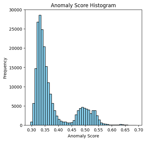
On Lines 90-99, we create a histogram of the anomaly scores using Matplotlib. The histogram has 50 bins with skyblue bars and black edges. The histogram helps us visualize the distribution of these scores, making it easier to identify potential anomalies.

Figure 8 shows the distribution of anomaly scores of the dataset.

**Figure 8:** Distribution of anomaly scores of the entire dataset after constructing the isolation forest (source: image by the author).

from sklearn.metrics import precision_score, recall_score

predictions =  (scores > 0.45).astype(np.int64)
# Calculate precision and recall
precision = precision_score(Y, predictions )
recall = recall_score(Y, predictions )

print("Total failures : ", Y.sum())
print("Detected failures : ", predictions.sum())
print("Correct failures : ", (predictions*Y).sum())
print("Missed failures : ", ((1-predictions)*Y).sum())

print(f'Precision: {precision:.2f}, Recall: {recall:.2f}, F1: {(2*precision*recall)/(precision + recall):.2f}')

Output:

Total failures :  14484
Detected failures :  24013
Correct failures :  11711
Missed failures :  2773
Precision: 0.49, Recall: 0.81, F1: 0.61

In this code snippet, we are evaluating the performance of our anomaly detection model using precision and recall metrics. On Line 100, we import the necessary functions precision_score and recall_score from sklearn.metrics. On Line 102, we generate binary predictions by thresholding the anomaly scores at 0.45, converting them to integers. On Lines 104 and 105, we calculate the precision and recall of our predictions against the actual target values (Y).

On Lines 107-110, we print out various statistics:

total number of failures in the dataset
number of detected failures
number of correctly detected failures
number of missed failures

Finally, on Line 112, we print the precision, recall, and F1 score (which is the harmonic mean of precision and recall).

What's next? We recommend PyImageSearch University.

Course information:
86 total classes • 115+ hours of on-demand code walkthrough videos • Last updated: October 2024
★★★★★ 4.84 (128 Ratings) • 16,000+ Students Enrolled

I strongly believe that if you had the right teacher you could master computer vision and deep learning.

Do you think learning computer vision and deep learning has to be time-consuming, overwhelming, and complicated? Or has to involve complex mathematics and equations? Or requires a degree in computer science?

That’s not the case.

All you need to master computer vision and deep learning is for someone to explain things to you in simple, intuitive terms. And that’s exactly what I do. My mission is to change education and how complex Artificial Intelligence topics are taught.

If you're serious about learning computer vision, your next stop should be PyImageSearch University, the most comprehensive computer vision, deep learning, and OpenCV course online today. Here you’ll learn how to successfully and confidently apply computer vision to your work, research, and projects. Join me in computer vision mastery.

Inside PyImageSearch University you'll find:

✓ 86 courses on essential computer vision, deep learning, and OpenCV topics
✓ 86 Certificates of Completion
✓ 115+ hours of on-demand video
✓ Brand new courses released regularly, ensuring you can keep up with state-of-the-art techniques
✓ Pre-configured Jupyter Notebooks in Google Colab
✓ Run all code examples in your web browser — works on Windows, macOS, and Linux (no dev environment configuration required!)
✓ Access to centralized code repos for all 540+ tutorials on PyImageSearch
✓ Easy one-click downloads for code, datasets, pre-trained models, etc.
✓ Access on mobile, laptop, desktop, etc.

Click here to join PyImageSearch University

Summary

In this blog post, we explore the concept of predictive maintenance and its importance in identifying potential equipment failures before they occur. We begin by discussing what predictive maintenance is and why anomaly detection plays a crucial role in this process. By detecting anomalies, we can predict when maintenance is needed, thus preventing unexpected breakdowns and reducing downtime.

We then delve into the Isolation Forest algorithm, a popular method for anomaly detection. This section covers the basics of Isolation Trees (iTrees) and how they are used to compute anomaly scores. By understanding how to build the forest and interpret these scores, we can effectively identify outliers that may indicate potential issues in the equipment.

Finally, we walk through the implementation of predictive maintenance using the Isolation Forest algorithm. This includes setting up the environment, preparing the data, building the Isolation Trees, and computing anomaly scores. We also cover the steps to build the forest and evaluate its performance, ensuring that our predictive maintenance system is both accurate and reliable.

Citation Information

Mangla, P. “Predictive Maintenance Using Isolation Forest,” PyImageSearch, P. Chugh, S. Huot, R. Raha, and P. Thakur, eds., 2024, https://pyimg.co/n41qw

@incollection{Mangla_2024_Predictive-Maintenance-Using-Isolation-Forest,
  author = {Puneet Mangla},
  title = {Predictive Maintenance Using Isolation Forest},
  booktitle = {PyImageSearch},
  editor = {Puneet Chugh and Susan Huot and Ritwik Raha and Piyush Thakur},
  year = {2024},
  url = {https://pyimg.co/n41qw},
}

To download the source code to this post (and be notified when future tutorials are published here on PyImageSearch), simply enter your email address in the form below!

Download the Source Code and FREE 17-page Resource Guide

Enter your email address below to get a .zip of the code and a FREE 17-page Resource Guide on Computer Vision, OpenCV, and Deep Learning. Inside you'll find my hand-picked tutorials, books, courses, and libraries to help you master CV and DL!

The post Predictive Maintenance Using Isolation Forest appeared first on PyImageSearch.

October 21, 2024 at 06:30PM
Click here for more details...

=============================
The original post is available in PyImageSearch by Puneet Mangla
this post has been published as it is through automation. Automation script brings all the top bloggers post under a single umbrella.
The purpose of this blog, Follow the top Salesforce bloggers and collect all blogs in a single place through automation.
============================

Puneet Mangla Python

Python Reader

Predictive Maintenance Using Isolation Forest : Puneet Mangla