Solving Ordinary Least Squares Using QR Decomposition : Puneet Mangla

April 21, 2025 April 21, 2025

Solving Ordinary Least Squares Using QR Decomposition
by: Puneet Mangla
blow post content copied from PyImageSearch
click here to view original post

Home

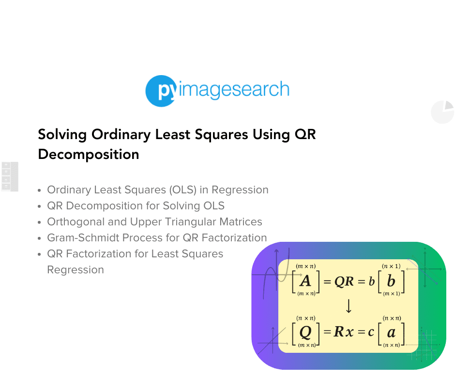
Solving Ordinary Least Squares Using QR Decomposition

In this tutorial, you will learn how to solve ordinary least squares regression using QR decomposition.

Ordinary Least Squares (OLS) is a fundamental method in statistics and machine learning for estimating the unknown parameters in a linear regression model. It provides the best linear unbiased estimator (BLUE) by minimizing the sum of the squared differences between the observed and predicted values. However, as datasets grow in size and complexity, ensuring numerical stability and efficiency in computations becomes paramount.

This is where QR Decomposition, a matrix factorization technique, comes into play. QR Decomposition allows us to transform the original problem into a more manageable form by decomposing the matrix of predictors into an orthogonal matrix $Q$ and an upper triangular matrix $R$ . This transformation not only enhances computational efficiency but also improves the numerical stability of the solution.

In this blog post, we will explore the theory behind QR Decomposition and its application in solving the OLS regression problem. Through detailed explanations and practical examples, you will gain a deeper understanding of how QR Decomposition can be leveraged to make linear regression more robust and efficient.

This lesson is the last in a 3-part series on Matrix Factorization:

To learn how to solve ordinary least squares regression using QR decomposition, just keep reading.

Looking for the source code to this post?

Overview of Ordinary Least Squares

Ordinary Least Squares (OLS) is one of the popular and widely adopted methods of estimating the unknown parameters in a linear regression model. Linear regression aims to model the relationship between a dependent variable $Y$ and one or more independent variables $X_i$ by fitting a linear equation to observed data.

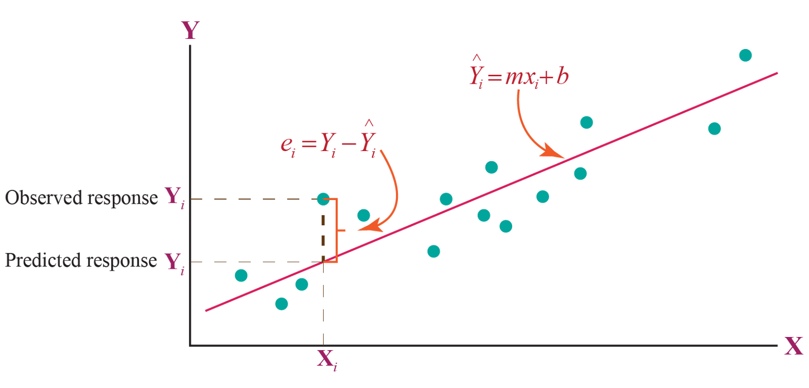
The OLS method achieves this by minimizing the sum of the squared differences between the observed values and the values predicted by the linear model, hence the name “least squares.”

The Linear Regression Model

The linear regression model (Figure 1) can be expressed as follows:

$y = X\beta + \epsilon$

where:

$y$ : the vector of observed values (dependent variable).
$X$ : the matrix of observed values of the independent variables (also called the design matrix).
$\beta$ : the vector of unknown parameters to be estimated.
$\epsilon$ : the vector of errors or residuals.

The goal of OLS is to find the parameter vector $\beta$ that minimizes the residual sum of squares (RSS), which is defined as follows:

$\text{RSS} = \displaystyle\sum_{i=1}^{n} (y_i - \hat{y}_i)^2 = (y - X\beta)^T(y - X\beta)$

where $\hat{y}$ represents the predicted values.

**Figure 1:** Ordinary Least Squares Regression (source: Cuemath).

Solving the Ordinary Least Squares Problem

To solve for $\beta$ , we set up the normal equations derived from simplifying the RSS minimization:

$(X^TX)\beta = X^Ty$

The solution to these equations gives us the OLS estimator for $\beta$ :

$\hat{\beta} = (X^TX)^{-1}X^Ty$

Directly computing the OLS estimator $\hat{\beta} = (X^TX)^{-1}X^Ty$ can be challenging due to numerical instability, computational complexity, and significant memory usage, especially for large or ill-conditioned matrices.

QR decomposition addresses these issues by decomposing $X$ into an orthogonal matrix $Q$ and an upper triangular matrix $R$ , enabling more stable and efficient computations. Instead of directly inverting $X^TX$ , QR decomposition transforms the problem into solving a simpler upper triangular system using back substitution (similar to an LU decomposition), thereby enhancing both numerical stability and computational efficiency.

What Is QR Decomposition?

QR decomposition (Figure 2) is a mathematical method used to factorize a matrix into two distinct matrices, $Q$ and $R$ , each with unique properties that make solving systems of linear equations more efficient and stable. This decomposition transforms a given matrix $A$ into the product of an orthogonal matrix $Q$ and an upper triangular matrix $R$ , such that

$A = QR$

**Figure 2:** QR Decomposition (source: DSC Spidal).

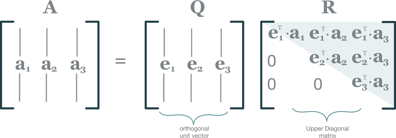
Orthogonal Matrix Q

An orthogonal matrix $Q$ (Figure 3) is a square matrix whose columns (or rows) are orthonormal vectors. This means that the dot product of any two distinct columns (or rows) of $Q$ is 0, and the norm of each column (or row) is 1.

Mathematically, a matrix $Q$ is orthogonal if:

$Q^TQ = QQ^T = I$

where $Q^T$ is the transpose of $Q$ , and $I$ is the identity matrix. The orthogonality property of $QQ$ ensures numerical stability and simplifies computations involving matrix inversion.

Upper Triangular Matrix R

The matrix $R$ is an upper triangular matrix, meaning that all the elements below the main diagonal are zero. The elements on and above the main diagonal can be non-zero. This triangular structure of $R$ makes it straightforward to solve systems of linear equations using back substitution (recall Lesson 1, where we saw how upper triangular matrices can help solve linear equations using back substitution).

Gram-Schmidt Process for QR Factorization

The Gram-Schmidt algorithm (Figure 4) is a method for obtaining the QR factorization of a matrix by orthogonalizing its columns. Here’s how it works:

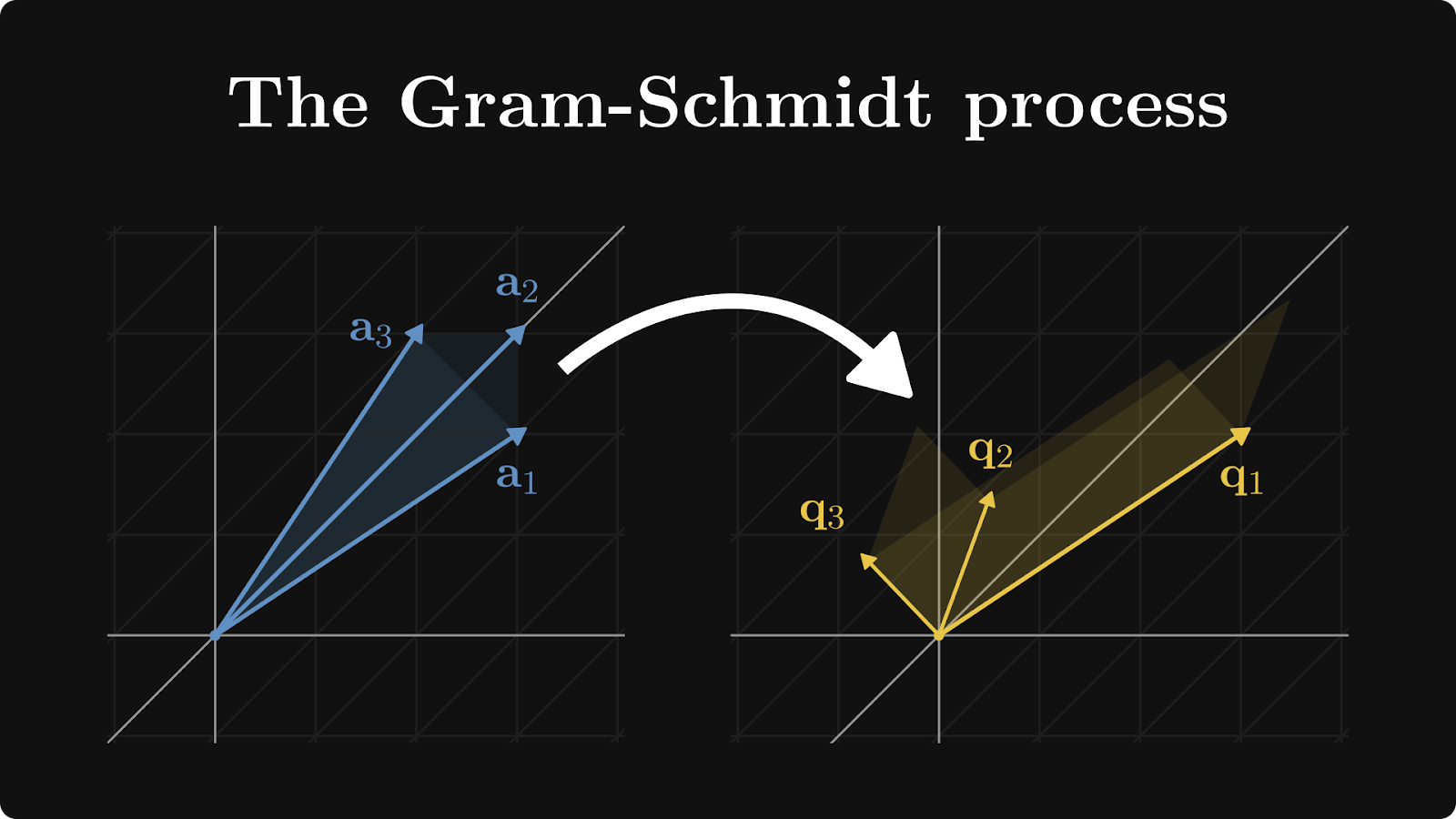
**Figure 4:** Gram-Schmidt process of orthogonalization (source: The Palindrome).

Gram-Schmidt Algorithm

Given a matrix $A$ with columns $a_1, a_2, \ldots, a_n$ , the goal is to decompose $A$ into an orthogonal matrix $Q$ and an upper triangular matrix $R$ .

Initialization

The first step is to start with the first column of $A$ , $a_1$ . Set

$q_1 = \displaystyle\frac{a_1}{\|a_1\|}$

where $\|a_1\|$ is the Euclidean norm of $a_1$ . This ensures $q_1$ , which is the first column of our $Q$ matrix, is a unit vector — as per the definition.

Orthogonalization

This step (Figure 5) involves transforming each subsequent column $a_i$ (where $i = 2, \ldots, n$ ) such that they are orthonormal to all previously transformed columns $q_j$ (where $j = 1, \ldots, i-1$ ):

First, we compute the projection of $a_i$ onto each of the previously computed orthonormal vectors $q_j$ for $j = 1, \ldots, i-1$ . The projection is given by:

$\text{proj}_{q_j} a_i = (a_i \cdot q_j) q_j$ .

Subtract these projections from $a_i$ to obtain the orthogonal component $u_i$ :

$u_i = a_i - \displaystyle\sum_{j=1}^{i-1} (a_i \cdot q_j) q_j$

Normalize $u_i$ to obtain the next orthonormal vector $q_j$ :

$q_i = \displaystyle\frac{u_i}{\|u_i\|}$

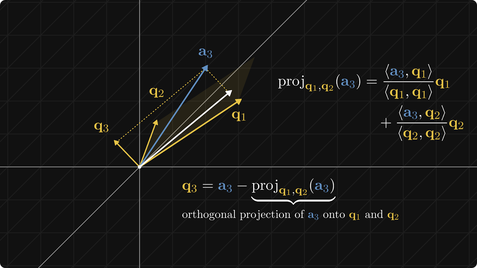**Figure 5:** Orthogonalization of column vectors of original matrix $A$ (source: The Palindrome).

Forming Matrices

Now that we have computed all orthonormal vectors $q_1, q_2, \ldots, q_n$ , we can begin by forming matrices $Q$ and $R$

The orthonormal vectors $q_1, q_2, \ldots, q_n$ form the columns of matrix $Q$ .
The coefficients used in the projections form the elements of the upper triangular matrix $R$ . Specifically, $R$ is constructed such that:

$R_{ij} = a_i \cdot q_j$ for $j \le i$ ,

and $R_{ij} = 0$ for $j > i$ .

Thus, we obtain the QR decomposition (Figure 6) $A = QR$ , where:

$Q = [q_1 \, q_2 \, \ldots \, q_n]$

$R$ is an upper triangular matrix with entries $R_{ij} = q_j \cdot a_i$ for $j \le i$

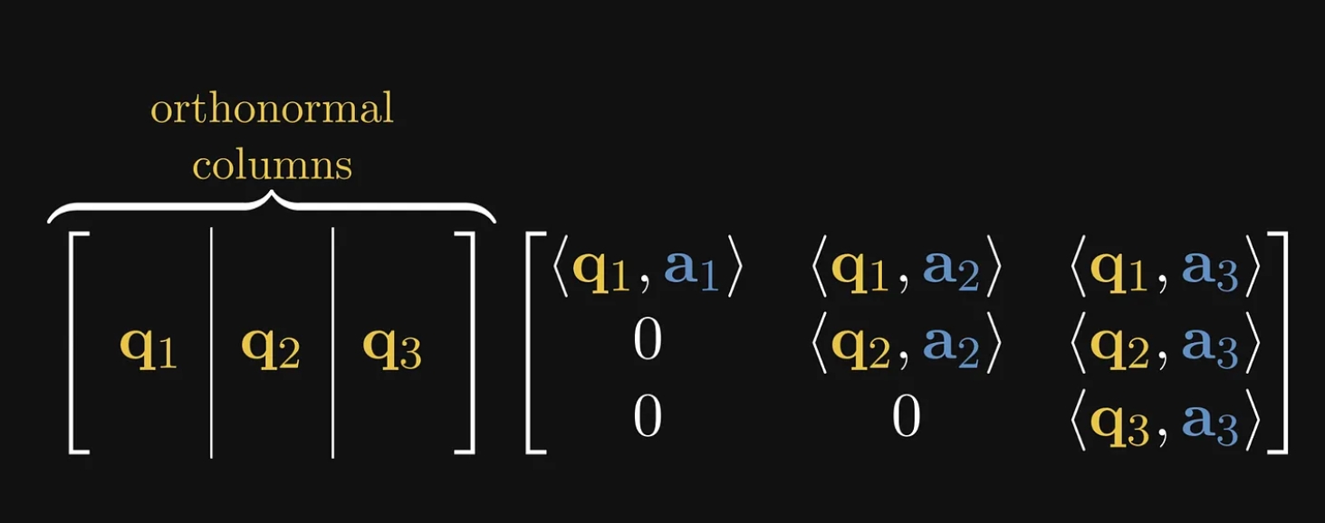**Figure 6:** Forming the $Q$ and $R$ matrices (source: The Palindrome).

Implementing the Gram-Schmidt Algorithm in Python

The code snippet below implements the Gram-Schmidt algorithm to perform the QR decomposition of a matrix. The code uses the NumPy library, which can be installed in your Python environment via pip install numpy.

import numpy as np

def gram_schmidt(A):
    """Perform QR factorization using the Gram-Schmidt process."""
    m, n = A.shape
    Q = np.zeros((m, n))
    R = np.zeros((n, n))

    for j in range(n):
        v = A[:, j]
        # Orthogonalization
        for i in range(j):
            R[i, j] = np.dot(Q[:, i], A[:, j])
            v = v - R[i, j] * Q[:, i]
       
        # Forming Q and R matrices
        R[j, j] = np.linalg.norm(v)
        Q[:, j] = v / R[j, j]

    return Q, R

# Example usage
A = np.array([[1, 2, 4], [3, 4, 7], [5, 6, 8]])
Q, R = gram_schmidt(A)

print("Matrix A:")
print(A)
print("\nMatrix Q:")
print(Q)
print("\nMatrix R:")
print(R)
print("\nVerifying A = QR:")
print(Q @ R)

Output:

Matrix A:
[[1 2 4]
 [3 4 7]
 [5 6 8]]

Matrix Q:
[[ 0.16903085  0.89708523 -0.40824829]
 [ 0.50709255  0.27602622  0.81649658]
 [ 0.84515425 -0.34503278 -0.40824829]]

Matrix R:
[[ 5.91607978  7.43735744 10.98700531]
 [ 0.          0.82807867  2.76026224]
 [ 0.          0.          0.81649658]]

Verifying A = QR:
[[1. 2. 4.]
 [3. 4. 7.]
 [5. 6. 8.]]

In this Python code, we start by importing numpy for matrix operations (Line 1). In the gram_schmidt function, we initialize zero matrices Q and R to store the orthogonal and upper triangular components (Lines 5-7).

We loop over each column of A, orthogonalize it by subtracting its projections on the previously computed orthonormal vectors, and store the coefficients in R (Lines 9-14). We then normalize the resulting vector to form the next orthonormal vector and store it in R and Q (Lines 17 and 18).

Finally, we return Q and R (Line 20). The example usage demonstrates how we can factorize a sample $3 \times 3$ matrix and verify $A = QR$ (Lines 23-33).

QR Factorization for Least Squares Regression

Transforming the Equations of Ordinary Least Squares Regression

The goal of OLS regression is to estimate the coefficient vector $\beta$ that minimizes the sum of squared residuals. This leads to the normal equations:

$(X^TX) \beta =X^Ty$

To simplify solving the above normal equations, we can leverage QR Factorization to decompose the matrix $X$ into two matrices: an orthogonal matrix $Q$ and an upper triangular matrix $R$ . The decomposition is expressed as follows:

$X = QR$

where:

$Q$ : an $m \times n$ orthogonal matrix ( $Q^TQ = I$ )
$R$ : an $n \times n$ upper triangular matrix

Using this decomposition, we can rewrite the normal equations as follows:

$R\beta = Q^Ty$

Solving the Transformed Equations

The transformed system $R\beta = Q^Ty$ is simpler to solve (than the original normal equation $(X^TX) \beta =X^Ty$ ) because $R$ is an upper triangular matrix, making it suitable for back substitution. The steps are as follows:

Compute $Q^Ty$ : Multiply the transpose of $Q$ by the vector $y$ , yielding a new vector.
Back Substitution: Solve the upper triangular system $\beta = Q^Ty$ using back substitution. Starting from the last row and moving upward, each variable $\beta_i$ can be solved sequentially.

Solving Ordinary Least Squares Using QR Factorization

In the Python code below, we solve an Ordinary Least Squares (OLS) regression problem using QR decomposition.

def ols_qr(X, y):
    """Solve OLS regression using QR decomposition."""
    # Perform QR decomposition
    Q, R = gram_schmidt(X)
   
    # Compute Q^T * y
    Qt_y = np.dot(Q.T, y)
   
    # Solve R * beta = Q^T * y using back substitution
    beta = np.zeros(R.shape[1])
    for i in reversed(range(R.shape[1])):
        beta[i] = (Qt_y[i] - np.dot(R[i, i+1:], beta[i+1:])) / R[i, i]
   
    return beta

# Example usage
X = np.array([[1, 1], [1, 2], [1, 3], [1, 4]])
y = np.array([6, 5, 7, 10])

beta = ols_qr(X, y)

print("Matrix X:")
print(X)
print("\nVector y:")
print(y)
print("\nEstimated coefficients (beta):")
print(beta)

Output:

Matrix X:
[[1 1]
 [1 2]
 [1 3]
 [1 4]]

Vector y:
[ 6  5  7 10]

Estimated coefficients (beta):
[3.5 1.4]

We start by defining the ols_qr function (Lines 34-47), which takes the design matrix X and the response vector y as inputs. Inside the function, we perform QR decomposition on X using the previously defined gram_schmidt function (Line 37). We then compute $Q^T y$ using the dot product of the transpose of Q and y (Line 40).

Next, we solve the triangular system $\beta = Q^T y$ using back substitution (Lines 43-45). This involves initializing the vector $\beta$ with zeros and iteratively solving for each coefficient in reverse order, from the last to the first.

In the example usage (Lines 50-60), we define a simple $4 \times 2$ design matrix X and a corresponding response vector y. We call the ols_qr function to compute the OLS regression coefficients $\beta$ .

What's next? We recommend PyImageSearch University.

Course information:
86+ total classes • 115+ hours hours of on-demand code walkthrough videos • Last updated: April 2025
★★★★★ 4.84 (128 Ratings) • 16,000+ Students Enrolled

I strongly believe that if you had the right teacher you could master computer vision and deep learning.

Do you think learning computer vision and deep learning has to be time-consuming, overwhelming, and complicated? Or has to involve complex mathematics and equations? Or requires a degree in computer science?

That’s not the case.

All you need to master computer vision and deep learning is for someone to explain things to you in simple, intuitive terms. And that’s exactly what I do. My mission is to change education and how complex Artificial Intelligence topics are taught.

If you're serious about learning computer vision, your next stop should be PyImageSearch University, the most comprehensive computer vision, deep learning, and OpenCV course online today. Here you’ll learn how to successfully and confidently apply computer vision to your work, research, and projects. Join me in computer vision mastery.

Inside PyImageSearch University you'll find:

✓ 86+ courses on essential computer vision, deep learning, and OpenCV topics
✓ 86 Certificates of Completion
✓ 115+ hours hours of on-demand video
✓ Brand new courses released regularly, ensuring you can keep up with state-of-the-art techniques
✓ Pre-configured Jupyter Notebooks in Google Colab
✓ Run all code examples in your web browser — works on Windows, macOS, and Linux (no dev environment configuration required!)
✓ Access to centralized code repos for all 540+ tutorials on PyImageSearch
✓ Easy one-click downloads for code, datasets, pre-trained models, etc.
✓ Access on mobile, laptop, desktop, etc.

Click here to join PyImageSearch University

Summary

This blog post tutorial provided a comprehensive guide on solving Ordinary Least Squares (OLS) regression using QR Decomposition, an efficient and numerically stable method of matrix factorization. The post explained the underlying principles of OLS, a method widely used in statistics and machine learning for estimating unknown parameters in a linear regression model. By minimizing the sum of squared differences between observed and predicted values, OLS aims to find the best linear unbiased estimators.

The tutorial delved into the mechanics of QR Decomposition, describing how it breaks down the design matrix into an orthogonal matrix $Q$ and an upper triangular matrix $R$ . This decomposition simplifies the linear regression problem, enhancing both computational efficiency and numerical stability. The post provided a step-by-step explanation of the Gram-Schmidt process used in QR factorization, illustrated with clear diagrams and a detailed Python code example.

Through practical examples and theoretical explanations, readers were equipped to implement QR Decomposition in solving the OLS regression, offering a deeper understanding of both the mathematical concepts and their application in real-world scenarios.

The blog concluded with a practical implementation of the QR Decomposition to solve the OLS problem using Python, providing readers with the tools to apply these techniques effectively in their data analysis projects. This tutorial is the final part of a 3-part series on matrix factorization. It is a valuable resource for those looking to enhance their understanding of advanced algebraic techniques in data science.

Citation Information

Mangla, P. “Solving Ordinary Least Squares Using QR Decomposition,” PyImageSearch, P. Chugh, S. Huot, and P. Thakur, eds., 2025, https://pyimg.co/z4vfe

@incollection{Mangla_2025_Solving-Ordinary-Least-Squares-Using-QR-Decomposition,
  author = {Puneet Mangla},
  title = ,
  booktitle = {PyImageSearch},
  editor = {Puneet Chugh and Susan Huot and Piyush Thakur},
  year = {2025},
  url = {https://pyimg.co/z4vfe},
}

To download the source code to this post (and be notified when future tutorials are published here on PyImageSearch), simply enter your email address in the form below!

Download the Source Code and FREE 17-page Resource Guide

Enter your email address below to get a .zip of the code and a FREE 17-page Resource Guide on Computer Vision, OpenCV, and Deep Learning. Inside you'll find my hand-picked tutorials, books, courses, and libraries to help you master CV and DL!

The post Solving Ordinary Least Squares Using QR Decomposition appeared first on PyImageSearch.

April 21, 2025 at 06:30PM
Click here for more details...

=============================
The original post is available in PyImageSearch by Puneet Mangla
this post has been published as it is through automation. Automation script brings all the top bloggers post under a single umbrella.
The purpose of this blog, Follow the top Salesforce bloggers and collect all blogs in a single place through automation.
============================

Puneet Mangla Python

Python Reader